Quick Links
With the growth in the adoption of DeFi, bonding curves have emerged as a pivotal mechanism for pricing tokens and managing liquidity. Although the concept is not new, it has gained popularity with DeFi. Bonding curves offer a mathematical approach to defining the relationship between the token supply and its price, enabling efficient and transparent market operations. Let’s dive into bonding curves, their function, their implications on token prices, and real-world examples, including concepts like slippage and impermanent loss.
What is a Bonding Curve?
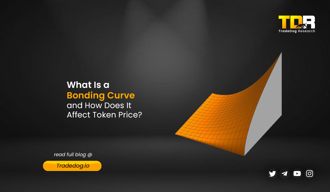
A bonding curve is a mathematical model that defines how the price of an asset changes in relation to its supply. Essentially, it is a smart contract that adjusts the price of a token according to a predefined formula as the token supply changes. The curve typically ensures that as more tokens are bought, the price increases, and as tokens are sold, the price decreases.
How Bonding Curves Work
Bonding curves are defined by formulas that determine token price (P) based on token supply (S). Common bonding curves include:
- Linear Curve: P(S)=k×S
- Exponential Curve: P(S)=k×e^S
- Logarithmic Curve: P(S)=k×log(S+1)
Bonding curves can take various mathematical forms, but one common type is the polynomial bonding curve. Here’s a basic example to illustrate how it works:
P(S)=k*(S^n)
- P(S)is the price of the token.
- S is the current supply of the token.
- K and n are constants that define the shape of the curve.
Let’s assume k=1 and n=2 for simplicity:
P(x)=x^2
In this scenario, if the supply of tokens is 10, the price per token would be:
P(10)=10^2=100
If the supply increases to 20, the price would be:
P(20)=20^2=400
As more tokens are purchased, the price rises steeply, incentivising early adopters to buy in when the price is low.
Use cases of Bonding Curves
Bonding curves are crucial for continuous liquidity and automated market-making in DeFi. They facilitate:
- Token minting and burning: Adjusting supply directly affects token pricing.
- Dynamic pricing models: Prices adjust based on real-time supply and demand.
- Decentralised governance: They can influence voting power in DAOs.
Some Applications in DeFi
- Aavegotchi employs bonding curves for GHST tokens, using them to manage supply dynamically.
- Uniswap and Balancer utilize variations of bonding curves in their liquidity pools, albeit with differing mechanisms:
- Uniswap uses a constant product formula, ensuring liquidity and price stability.
- Balancer allows for custom pool configurations, including multiple tokens with adjustable weights.
Challenges
Implementing bonding curves involves extensive modelling, security audits, and compliance analysis. Ensuring the curves are neither too steep nor too shallow is crucial to avoid price manipulation. Additionally, the regulatory landscape for bonding curves is evolving, requiring careful legal consideration.
Bonding Curves: Well aligned with the ethos of Decentralisation
Bonding curves offer a transparent and dynamic method for pricing tokens in DeFi, embedding liquidity directly into the token’s smart contract. While they provide significant advantages, including automated liquidity and real-time price adjustments, they also pose challenges that require careful design and regulation.
By understanding bonding curves, investors and developers can leverage their potential to optimize DeFi strategies and enhance market efficiency.


